GAMS: Piecewise linear functions with SOS2 variables

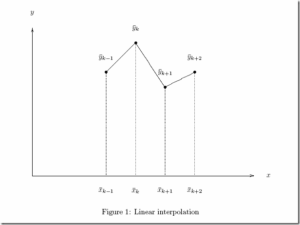
Sometimes we need to represent a piecewise linear function, like:

This can be modeled with the following:

Equation (1) is ! called the “reference row”, equation (2) the “function row” and equation (3) the “convexity row”. Many MIP solvers have so-called SOS2 facilities: special ordered sets of type 2. The lambda variables form a SOS2 set, so this makes using this very simple (it is possibly to simulate this with extra binary variables). In GAMS this looks like:

variables y,x;
sos2 variables lambda(k);

equations refrow, funrow, convexity;

refrow.. x =e= sum(k, lambda(k)*xbar(k));
funrow.. y =e= sum(k, lambda(k)*ybar(k));
convexity.. sum(k, lambda(k)) =e= 1;

Notes:

• It is important to keep the “set-index” last. See the fragment of a model I am working at now:

defq(i,t).. q(i,t) =e= sum(ic(i,c)! , lambda(i,t,c)*xpoints(c));

d efcost(i,t)..  cost(i,t) =e= sum(ic(i,c), lambda(i,t,c)*ypoints(i,c));

convex(i,t)..  sum(ic(i,c),lambda(i,t,c)) =e= 1;

Here we need to keep c last in variable lambda. This makes sure we have i × t sets with c members. In this case c is dependent on i through the set ic(i,c).

• AMPL has special language constructs to make this even easier.
• MS Solver Foundation also has added SOS2 support.
• GAMS has no facility to specify the reference weights (they are usually automatically generated to be 1,2,…).  Of course in many cases I can not make a good use of reference weights anyway, as I would not know any better values.

Linear Functions